
Computational Geodynamics: Mathematical Models
Sections
\[ \require{color} \newcommand{\dGamma}{\mathbf{d}\boldsymbol{\Gamma}} \newcommand{\erfc}{\mbox{\rm erfc}} \newcommand{\Red}[1]{\textcolor[rgb]{0.7,0.0,0.0}{#1}} \newcommand{\Green}[1]{\textcolor[rgb]{0.0,0.7,0.0}{ #1}} \newcommand{\Blue}[1]{\textcolor[rgb]{0.0,0.0,0.7}{ #1}} \newcommand{\Emerald}[1]{\textcolor[rgb]{0.0,0.7,0.3}{ #1}} \]
Let us start by deriving the equations of motion, energy balance and so on through a conservation principle. This will give a useful insight into the different forms of the equations which we will later encounter.
A general conservation law does not distinguish the quantity which is being conserved – it is a mathematical identity. Consider a quantity \( \phi \) / unit mass which is carried around by a fluid. We can draw an arbitrary volume, \( \Omega \) to contain some amount of this fluid at a given time. We label the surface of the volume \( \Omega \) as \( \Gamma \), and define an outward surface normal vector \( \dGamma \) which is normal to the tangent plane of an infinitesimal element of the surface and has a magnitude equal to the area of this element.

We also define a source/sink term, \(H\) / unit mass which generates/consumes the quantity \( \phi \), and a flux term, \(\mathbf{F}\) which occurs across the surface when the fluid is stationary (e.g. this might represent diffusion of \( \phi \)). The rate of change of \( \phi \) is given by combining the contribution due to the source term, the stationary flux term, and the effect of motion of the fluid.
\begin{equation} \frac{d}{dt} \int _ {\Omega} \rho \phi d\Omega = - \int _ {\Gamma} \mathbf{F} \cdot \dGamma + \int _ {\Omega} \rho H d\Omega - \int _ {\Gamma} \rho \phi \mathbf{v} \cdot \dGamma \label{eq:1} \end{equation}
where the final term is the change due to the fluid carrying \( \phi \) through the volume. Fluxes are positive outward (by our definition of \( \dGamma \)), so a positive flux reduces \( \phi \) within \( d\Omega \) and negative signs are needed for these terms.
We can generally use Gauss’ theorem to write surface integrals as volume integrals:
\begin{equation} \nonumber \int _ {\Gamma} \phi \mathbf{u} \cdot \dGamma = \int _ {\Omega} \nabla \cdot (\phi \mathbf{u}) d\Omega \end{equation}
The test surface, \( \Gamma \), and volume, \( \Omega \) are assumed to be_fixed in the lab reference frame_ so that the order of integration and differentiation can be interchanged
\begin{equation} \nonumber \frac{d}{dt} \int_\Omega \rho \phi d\Omega = \int _ \Omega \frac{\partial \rho \phi}{\partial t} d \Omega \end{equation}
Allowing us to write
\begin{equation} \nonumber \int_{\Gamma} \mathbf{F} \cdot \dGamma + \int _ {\Gamma} \rho \phi \mathbf{v} \cdot \dGamma = \int _ {\Omega} \nabla \cdot (\mathbf{F} + \rho \phi \mathbf{v}) d\Omega \end{equation}
so that we rewrite the general conservation equation as
\begin{equation} \int_{\Omega} \left[ \frac{d \rho \phi}{dt} + \nabla \cdot (\mathbf{F} + \rho \phi \mathbf{v}) -\rho H \right] d\Omega=0 \label{eq:cons1}) \end{equation}
We can now appeal to the fact that this conservation law holds regardless of our particular choice of volume \( \Omega \) and, therefore, the integral above can only be zero for arbitrary \( \Omega \) if the enclosed term is zero everywhere, i.e.
\begin{equation} \frac{d \rho \phi}{dt} + \nabla \cdot (\mathbf{F} + \rho \phi \mathbf{v}) -\rho H =0 \label{eq:cons2} \end{equation}
This is a general conservation rule for any property \( \phi \) of a moving fluid. We now consider various quantities that may be transported and develop specific conservation laws.
Conservation of mass
In this case\( \phi = 1 \) (since \(\int_\Omega \rho d\Omega \rightarrow \mbox{mass}\)), \(\mathbf{F} = H = 0\).
Thus, equation (\ref{eq:cons2}) gives
\begin{equation} \Red{\frac{\partial \rho}{\partial t} + \nabla \cdot \rho \mathbf{v} = 0} \label{eq:masscons} \end{equation}
Conservation of (heat) energy
The thermal energy / unit mass is \(C_p T\) and the conductive heat flux \(\mathbf{F}\) is given by \( \mathbf{F} = -k \nabla T\), where \(k\) is the thermal conductivity. Then the general conservation law of \( (\ref{eq:cons2}) \) reduces to
\begin{equation} \nonumber \frac{\partial (\rho C_p T)}{\partial t} + \nabla \cdot \left(-k \nabla T + \rho C_p T \mathbf{v}\right) - \rho H = 0 \end{equation}
Rearranging with some foresight gives the following: \begin{equation} \nonumber \frac{C_p T}{\rho} \left[ \frac{\partial \rho}{\partial t} + \nabla \cdot \rho \mathbf{v} \right] + \frac{\partial C_p T}{\partial t} + \mathbf{v} \cdot \nabla C_p T = \frac{1}{\rho} \nabla \cdot k \nabla T + H \end{equation}
Where the term in square brackets is simply the statement of mass conservation which vanishes identically. The constant density assumption is just to simplify the discussion at this point and will have to be revisited later in the context of thermal convection where density changes drive the flow.
If the heat capacity, \(C_p\) and thermal conductivity, \(k \) are constants, then the conservation equation becomes \begin{equation} \nonumber \Red{ \left( \frac{\partial T}{\partial t} + \mathbf{v} \cdot \nabla T \right)= \kappa \nabla ^ 2 T + \frac{H}{C _ p} } \label{eq:energycons} \end{equation}
where \(\kappa\) is the thermal diffusivity, \(\kappa = k/\rho C_p\). This equation is linear provided that the velocity field is specified and is independent of \(T\). Clearly this is generally not true because mantle circulation is driven by thermal buoyancy.
A new bit of notation has been defined in the process of this derivation. The meaning of the \(\mathbf{v} \cdot \nabla\) operator is
\begin{equation} \nonumber \mathbf{v} \cdot \nabla \equiv v _ j \frac{\partial}{\partial x _ j} \end{equation}
For later reference, this is how it looks: \begin{equation} \nonumber (\mathbf{v} \cdot \nabla) T = v _ 1 \frac{\partial T}{\partial x _ 1} + v _ 2 \frac{\partial T}{\partial x _ 2} + v _ 3 \frac{\partial T}{\partial x _ 3} \end{equation}
The Laplacian, \(\nabla ^ 2\), is this expression (for scalar \(T\)) \begin{equation} \nonumber \nabla ^ 2 T \equiv \frac{\partial ^ 2 T}{\partial x _ 1 ^ 2} + \frac{\partial ^ 2 T}{\partial x _ 2 ^ 2} + \frac{\partial ^ 2 T}{\partial x _ 3 ^ 2} \end{equation}
Conservation of momentum
Momentum is a vector quantity, so the form of (\ref{eq:cons1}) is slightly different. The source term in a momentum equation represents a force, and the surface flux term represents a stress.
\begin{equation}
\frac{d}{dt}\int _ {\Omega} \rho \mathbf{v} d\Omega =
- \int _ {\Omega} \rho g \hat{\mathbf{z}} d\Omega
+ \int _ {\Gamma} \boldsymbol{\sigma} \cdot \dGamma -
\int _ {\Gamma} \rho \mathbf{v} (\mathbf{v} \cdot \dGamma)
\label{eq:momcons1}
\end{equation}
Gravity acts as a body force in the vertical direction, \(\hat{\mathbf{z}}\). We have introduced the stress tensor, \(\boldsymbol{\sigma}\); the force / unit area exerted on an arbitrarily oriented surface with normal \(\hat{\mathbf {n}}\) is
\begin{equation} \nonumber f _ i = \sigma _ {ij} n _ j \end{equation}
The application of Gauss’ theorem, and using the arbitrary nature of the chosen volume to require the integrand to be zero, as before, gives
\begin{equation} \frac{\partial}{\partial t}(\rho \mathbf{v}) +\rho g \hat{\mathbf{z}} - \nabla \cdot \sigma + \nabla \cdot (\rho \mathbf{v} \mathbf{v}) = 0 \label{eq:momcons2} \end{equation}
Vector notation allows us to keep a number of equations written as one single equation. However, at this point, keeping the equations in vector notation makes the situation more confusing. Particularly, the last term of equation \( (\ref{eq:momcons2}) \) stretches the current notation rather too much. Instead, we consider the individual components of momentum, each of which must satisfy the conservation law independently In index notation, equation (\ref{eq:momcons2}) is written as
\begin{equation} \nonumber \Green{\frac{\partial \rho v _ i}{\partial t}} + \rho g \delta _ {i3} - \frac{\partial \sigma _ {ij}}{\partial x _ j} + \Blue{\frac{\partial(\rho v _ i v _ j)}{\partial x _ j}} = 0 \label{eq:momindx} \end{equation}
where the troublesome final term is now unambiguous. Repeated indeces in each term are implicitly to be summed. \( \delta _ {ij}\) is the kronecker delta which obeys:
\begin{equation} \nonumber
\delta _ {ij} = \begin{cases}
0 & \text{if $i \neq j$}, \
1 & \text{if $i = j$}.
\end{cases}
\end{equation}
With some foresight, we expand the derivatives of products of two terms and gather up some of the resulting terms: \begin{equation} \nonumber v _ i \left[\Green{\frac{\partial \rho}{\partial t}} + \Blue{ \frac{\partial \rho v _ j}{\partial x _ j}} \right] + \Green{\rho \frac{\partial v _ i}{\partial t}} + \Blue{\rho v _ j \frac{\partial v _ i}{\partial x _ j}} = \frac{\partial \sigma _ {ij}}{\partial x _ j} -\rho g \delta _ {i3} \end{equation}
The term in square brackets is, in fact, a restatement of the conservation of mass derived above and must vanish. The remaining terms can now be written out in vector notation as
\begin{equation} \nonumber \Red{ \rho \left( \frac{\partial \mathbf{v}}{\partial t} + (\mathbf{v} \cdot \nabla) \mathbf{v} \right) = \nabla \cdot \boldsymbol{\sigma} - g\rho\hat{\mathbf{z}} } \label{eq:momcons3} \end{equation}
Note: The \(\mathbf{v} \cdot \nabla \) notation we introduced earlier is now an operator on a vector. In this context, the \(\mathbf{v} \cdot \nabla \) operator acts on each component of the vector independently. Written out it looks like this:
\begin{equation} \nonumber
\begin{split}
(\mathbf{v} \cdot \nabla) \mathbf{u} =
& \hat{\boldsymbol{\imath}} \left( v _ 1 \frac{\partial u _ 1}{\partial x _ 1} +
v_2 \frac{\partial u _ 1}{\partial x _ 2} + v_3 \frac{\partial u _ 1}{\partial x _ 3} \right) \
& \hat{\boldsymbol{\jmath}} \left( v_1 \frac{\partial u_2}{\partial x_1} +
v_2 \frac{\partial u _ 2}{\partial x _ 2} + v _ 3 \frac{\partial u _ 2}{\partial x _ 3} \right) \
& \hat{\boldsymbol{k}} \left( v_1 \frac{\partial u_3}{\partial x_1} +
v_2 \frac{\partial u _ 3}{\partial x _ 2} + v _ 3 \frac{\partial u _ 3}{\partial x _ 3} \right) \
\end{split}
\end{equation}
Constitutive Laws
The formulation above is quite general, and can be extended where necessary to include conservation laws for additional physical variables (for example, angular momentum, electric current). Specific to the type of material which is deforming is the constitutive law which describes the stress. In the case of an incompressible fluid, the stress is related to strain rate through a viscosity, \(\eta\), and to the pressure, \(p\). Incompressibility is expressed as
\begin{equation} \nonumber \nabla \cdot \mathbf{u} = 0 \end{equation}
This is a tighter constraint than mass conservation and emerges from equation (\ref{eq:masscons}) when \( \rho \) is assumed to be constant. With this assumption, the constitutive law is written (A derivation for this is in Landau & Lifschitz).
\begin{equation} \nonumber \sigma _ {ij} = \eta \left( \frac{\partial v _ i}{\partial x _ j} + \frac{\partial v _ j}{\partial x _ i}\right) - p\delta _ {ij} \end{equation}
If the viscosity is constant, then we can substitute the constitutive law into the stress-divergence term of the momentum conservation equation. In index notation once again,
\begin{equation} \nonumber
\begin{split}
\nabla \cdot \boldsymbol{\sigma} & =
\frac{\partial}{\partial x _ j} \eta
\left( \frac{\partial v _ i}{\partial x _ j} + \frac{\partial v _ j}{\partial x _ i} \right)
- \frac{\partial p}{\partial x _ j} \delta _ {ij}
& = \eta \frac{\partial^2 v_i}{\partial x _ j \partial x _ j} +
\eta \frac{\partial^2 v _ j}{\partial x _ i \partial x _ j} -
\frac{\partial p}{\partial x _ i}
& = \eta \nabla^2 \mathbf{v} +
\eta \Green{\nabla (\nabla \cdot \mathbf{v})} - \nabla p
\end{split}
\end{equation}
the second term in this final form must vanish because of the incompressibility assumption, so the momentum conservation equation becomes
\begin{equation} \Red{ \rho \left( \frac{\partial \mathbf{v}}{\partial t} + (\mathbf{v} \cdot \nabla) \mathbf{v} \right) = \eta \nabla^2 \mathbf{v} - \nabla p - g\rho\hat{\mathbf{z}} } \label{eq:navstokes} \end{equation}
This is the Navier-Stokes equation. Once again some new notation has shown up uninvited. The Laplacian operator \(\nabla ^ 2\) is defined (in a scalar context) as
\begin{equation} \nonumber
\begin{split}
\nabla ^ 2 \phi & = \nabla \cdot \nabla \phi \
& = \frac{\partial ^ 2 \phi}{\partial x ^ 2} +
\frac{\partial ^ 2 \phi}{\partial y ^ 2} +
\frac{\partial ^ 2 \phi}{\partial z ^ 2}
\;\;\; \textrm{(Cartesian)}
\end{split}
\end{equation}
and in a vector context as
\begin{equation} \nonumber
\begin{split}
\nabla^2 \mathbf{u} & = \nabla \nabla \cdot \mathbf{u} - \nabla \times (\nabla \times \mathbf{u})
& = \mathbf{i} \nabla \cdot \nabla u_x +
\mathbf{j} \nabla \cdot \nabla u_y +
\mathbf{k} \nabla \cdot \nabla u_z
\;\;\; \text{(Cartesian)}
\end{split}
\end{equation}
In Cartesian coordinates, the Laplacian operator has a simple form, and the vector Laplacian is simply the scalar operator applied in each direction. In other coordinate systems this operator becomes substantially more elaborate.
Boussinesq Approximation, Equation of State, Density Variations
The equation which relates pressure, temperature and density is known as the equation of state. For the equations derived so far, we have specified an incompressible fluid, for which no density variations are possible. However, we have also included a source term for momentum which relies on gravity acting on density variations.
This conflict is typical of fluid mechanics: simplifying assumptions if taken to their logical limit imply no motion or some other trivial solution to the equations.
In this case, we make the assumption that density changes are typically small relative to the overall magnitude of the density itself. Terms which are scaled by density can therefore assume that it is a large constant value. Terms which contain gradients of density or density variations should consider the equation of state. This is the Boussinesq approximation and is only a suitable appropriation for nearly- incompressible fluids. In the Navier-Stokes equation, the hydrostatic pressure does not influence the velocity field at all. Only \textit{differences} in density drive fluid flow, and so the sole term in which density needs to be considered variable is that of the gravitational body forces.
In the case of density variations due to temperature, the equation of state is simply \[ \begin{equation} \rho = \rho_0 \left(1 - \alpha ( T-T_0 )\right) \label{eq:state} \end{equation} \]
where \(\rho_0\) is the density at a reference temperature \(T_0\). \( \alpha \) is the coefficient of thermal expansion. It is generally much smaller than one, making the Boussinesq approximation a reasonable choice. The energy and momentum conservation equations thus become coupled through the term
\begin{equation} \nonumber g\rho\hat{\mathbf{z}} = g \rho_0 \left(1 - \alpha(T-T_0)\right) \end{equation}
Density variations due to pressure produce a perfectly vertical, isotropic forcing term on the momentum conservation equation. In the steady state case, this is balanced by the hydrostatic pressure gradient. (The isotropic term does not contribute at all the the deviatoric part of the stress equation and thus cannot induce steady flow). We therefore ignore the vertical density gradient due to the fluid overburden.
Another density variation is that which results from variation in chemical composition from one fluid element to another. This is the case where two immiscible fluids live in the same region. Now density variations might be large – the fluid domains must be considered separately.
Advection and the Lagrangian Formulation
We have seen the \(\mathbf{v} \cdot \nabla \) operator a number of times now. The presence of this term causes major difficulties in continuum mechanics since it introduces a strong non-linearity into the momentum equation. It is this term which produces turbulence in high speed flows etc.
This term is the ‘advection’ term which accounts for the passive transport of information (temperature, momentum, by the motion of the fluid. Advection also presents some serious headaches in numerical methods and has spawned entire literatures devoted to efficient and accurate solution methods.
One obvious way to avoid the problem of advection is to consider an elemental volume of space which {\em moves with the fluid}. The surface flux term from equation \( (\ref{eq:cons1}) \) vanishes immediately.
Mathematically, we introduce a new notation (of course), as follows:
\begin{equation} \nonumber \frac{D \phi}{D t} = \frac{d}{dt} \phi[x _ 1(t),x _ 2(t),x _ 3(t),t] \end{equation}
where the change in the reference position \( (x _ 1(t),x _ 2(t),x _ 3(t)) \) is governed by the local flow velocity: \begin{equation} \nonumber \frac{d x _ 1}{d t} = v _ 1 \;\;\; \frac{d x _ 2}{d t} = v _ 2 \;\;\; \frac{d x _ 3}{d t} = v _ 3 \end{equation}
which keeps the reference point moving with the fluid. Differentiating gives
\begin{align}
\frac{D \phi}{D t} &= \frac{\partial \phi}{\partial t}
\frac{\partial \phi}{\partial x _ 1}\frac{d x _ 1}{d t} +
\frac{\partial \phi}{\partial x _ 2}\frac{d x _ 2}{d t} +
\frac{\partial \phi}{\partial x _ 3}\frac{d x _ 3}{d t} \nonumber \
\textrm{and so leads to} \;\;\;
\frac{D \phi}{D t} &= \frac{\partial \phi}{\partial t}
v_1 \frac{\partial \phi}{\partial x_1} +
v_2 \frac{\partial \phi}{\partial x_2} +
v_3 \frac{\partial \phi}{\partial x_3} \nonumber \
\textrm{which is equivalent to} \;\;\;
\frac{D \phi}{D t} &= \frac{\partial \phi}{\partial t} + (\mathbf{v} \cdot \nabla) \phi
\end{align}
If we think of \( \phi \) as the concentration of a dye in the fluid, then the above is a conservation equation assuming the dye does not diffuse and has no sources or sinks. Viewed from a reference frame locked to a particular fluid element, the energy conservation equation becomes
\begin{equation} \nonumber % \rho ?? \frac{D T}{Dt} = \kappa \nabla^2 T + \frac{H}{C_p} \end{equation}
and the momentum conservation equation now becomes \[ \begin{equation} \nonumber \rho %% ? \frac{D \mathbf{v} }{D t} = \eta \nabla^2 \mathbf{v} - \nabla P - g\rho\hat{\mathbf{z}} \end{equation} \]
This is a considerably more compact way of writing the equations, but we have only really succeeded in hiding the nasty term under the rug, since it is now necessary to use a coordinate system which is locked into the fluid and rapidly deforms as the fluid flows. Before long, the coordinate system is unimaginably complex – the advection problem returns in another guise. This formulation is known as the Lagrangian formulation and contrasts with the Eulerian viewpoint which is fixed in space.
From the numerical point of view, however, this approach can have some distinct advantages. The computer can often track the distorted coordinate system far better than it can handle successive applications of the \( \mathbf{v} \cdot \nabla \) operator at a fixed point in space. We will return to this point later.
Non-dimensional equations & dimensionless numbers
Before too long it would be a good idea to get a feeling for the flavour of these equations which continual rearrangements will not provide — it is necessary to examine some solutions.
First of all, however, it is a good idea to make some simplifications based on the kinds of problems we will want to attack. The first thing to do, as is often the case when developing a model, is to test whether any of the terms in the equations are negligibly small, or utterly dominant. This is done by, essentially, dimensional analysis.
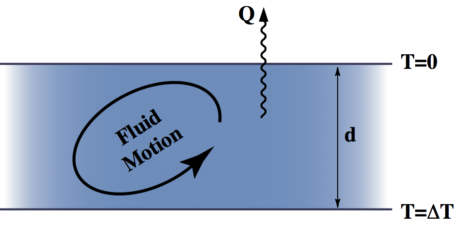
Now we consider some `typical values’ for the independent dimensions of the system (mass, length, time, temperature, that sort of thing) which can be used to rescale the standard units. We rescale all lengths by the depth of the fluid, \( d \) (e.g. mantle thickness or depth of fluid in a lab tank), time according to the characteristic time for diffusion of heat, and temperature by the temperature difference across the depth of the layer. Obviously these choices are dependent on the problem in question but this exercise is a common one in fluid dynamics and provides a useful first step in the assault on the problem
Various scalings result, with the new variables indicated using a prime (\(‘\)).
\begin{equation} \nonumber
\begin{array}{llll}
x = d.x’ & \partial / \partial x = (1/d) \partial / \partial x’ & \nabla = (1/d) \nabla ‘ \
t = (d^2/\kappa) t’ & \partial / \partial t = (\kappa/d^2) \partial / \partial t’ & \
T = \Delta T T’ & & \
v = (\kappa / d) v’ && \
p= p_0 + (\eta \kappa / d^2) p’
\end{array}
\end{equation}
where \begin{equation} \nonumber \nabla p _ 0 = - g \rho_0 \end{equation}
Substituting for all the existing terms in the Navier-Stokes equation (\ref{eq:navstokes}) using the equation of state for thermally induced variation in density (\ref{eq:state}) gives: \begin{equation} \nonumber \frac{\rho_0 \kappa}{d^2} \frac{D}{Dt’} \left( \frac{\kappa}{d} \mathbf{v}’ \right) = \frac{\eta}{d^2} \acute{\nabla}^2 \left( \frac{\kappa}{d} \mathbf{v}’ \right) - \frac{\eta \kappa}{d^3} \acute{\nabla} p’ + g \rho_0 \alpha \Delta T T’ \hat{\mathbf{z}} \end{equation}
Collecting everything together gives \begin{equation} \nonumber \frac{\rho_0 \kappa^2}{d^3} \frac{D\mathbf{v}’}{Dt’} = \frac{\eta \kappa}{d^3} \acute{\nabla}^2 \mathbf{v}’ - \frac{\eta \kappa}{d^3} \acute{\nabla} p’ + g \rho_0 \alpha \Delta T T’ \hat{\mathbf{z}} \end{equation}
Divide throughout by \(\eta \kappa / d^3\) gives
\begin{equation} \nonumber \frac{\rho \kappa}{\eta} \frac{D\mathbf{v}’}{Dt’} = \acute{\nabla} ^ 2 \mathbf{v}’ - \acute{\nabla} p’ + \frac{g \rho _ 0 \alpha \Delta T d ^ 3}{\kappa \eta} T’ \hat{\mathbf{z}} \end{equation}
where we can bundle up the coefficients into two dimensionless constants
\begin{equation} \frac{1}{\textrm{Pr}} \frac{D \mathbf{v}’ }{Dt’ } = \acute{\nabla}^2 \mathbf{v}’ - \acute{\nabla} p’ + \textrm{ Ra} T’ \hat{\mathbf{z}} \end{equation}
\(\rm Pr\) is known as the Prandtl number, and \(\rm Ra\) is known as the Rayleigh number. By choosing to scale the equations (and this is still perfectly general as we haven’t forced any particular choice of scaling yet), we have condensed the different physical variable quantities into just two numbers. The benefit of this procedure is that it tells us how different quantities trade off against one another. For example, we see that if the density doubles, and the viscosity doubles, then the solution should remain unchanged.
In fact, the main purpose of this particular exercise is about to be revealed. The value of mantle viscosity is believed to lie somewhere between \(10^{19}\) and \(10^{23}\) \({\rm Pa . s}\), the thermal diffusivity is around \(10 ^ {-6}{\rm m}^2{\rm s}^{-1}\), and density around \(3300 {\rm kg . m}^{-3}\). This gives a Prandtl number greater than \(10^{20}\). Typical estimates for the Rayleigh number are between \(10^6\) and \(10^8\) depending on the supposed depth of convection, and the uncertain mantle viscosity. The fact that the constants may all vary with temperature and pressure increases the difficulty in specifying a meaningful single value of the Rayleigh number for any planet.
Obviously, the time-dependent term (accelerations or the importance of inertia) can be neglected for the mantle, since it is at least twenty orders of magnitude smaller than other terms in the equations. The benefit of this is that the nasty advection term for momentum is eliminated – flow in the mantle is at the opposite extreme to turbulent flow. The disadvantage is that the equations now become non-local: changes in the stress field are propogated instantly from point to point which can make the equations a lot harder to solve. This can be counter-intuitive but the consequences are important when considering the dynamic response of the Earth to changes in, for example, plate configurations.
Incidentally, a third, independent dimensionless number can be derived for the thermally driven flow equations. This is the Nusselt number \begin{equation} \nonumber {\rm Nu} = \frac{Q}{k\Delta T} \end{equation}
and is the ratio of actual heat transported by fluid motions in the layer compared to that transported conductively in the absence of fluid motion.
All other dimensionless quantities for this system can be expressed as some combination of the Nusselt, Rayleigh and Prandtl numbers. The Prandtl number is a property of the fluid itself – typical values are: air, \( \sim \) 1; water, \( \sim\) 6; non-conducting fluids \(10^3\) or more; liquid metal, \( \sim \) 0.1. Rayleigh number and Nusselt number are both properties of the chosen geometry.
Stream function / Vorticity Notation
For incompressible flows in two dimensions it can be very convenient to work with the stream-function – a scalar quantity which defines the flow everywhere. Another quantity much beloved of fluid dynamicists is the vorticity. Although the application of such quantities to deformation of the solid planets is actually quite limited, it is still useful for exploring the basic fluid dynamics of the large scale flow.
Streamfunction
The stream function is the scalar quantity, \( \psi \), which satisfies \[ \begin{equation} v_1 = -\frac{\partial \psi}{\partial x_2} \;\;\; v_2 = \frac{\partial \psi}{\partial x_1} \label{eq:strmfn} \end{equation} \] so that, automatically, \[ \begin{equation} \nonumber \frac{\partial v_1}{\partial x_1} + \frac{\partial v_2}{\partial x_2} = 0 \end{equation} \]
Importantly, computing the following \[ \begin{equation} \nonumber (\mathbf{v} \cdot \nabla) \psi = v_1 \frac{\partial \psi}{\partial x_1} + v_2 \frac{\partial \psi}{\partial x_2} = \frac{\partial \psi}{\partial x_2} \frac{\partial \psi}{\partial x_1} - \frac{\partial \psi}{\partial x_1} \frac{\partial \psi}{\partial x_2} = 0 \end{equation} \] tells us that \(\psi\) does not change due to advection – in other words, contours of constant \(\psi\) re streamlines of the fluid.
Provided we limit ourselves to the xy plane, it is possible to think of equation (\ref{eq:strmfn}) as
\begin{equation} \nonumber \mathbf{v} = \nabla \times (\psi \hat{\mathbf{k}}) \end{equation}
This form can be used to write down the2D axisymetric version of equation (\ref{eq:strmfn}) at once
\begin{eqnarray} u_r = -\frac{1}{r}\frac{\partial \psi}{\partial \theta} & & u_\theta = \frac{\partial \psi}{\partial r} \end{eqnarray}
which automatically satisfies the incompressibility condition in plane polar coordinates
\begin{equation} \nonumber \frac{1}{r}\frac{\partial}{\partial r}(ru_r) + \frac{1}{r}\frac{\partial u_\theta}{\partial \theta} = 0 \end{equation}
Vorticity
Vorticity is defined by
\begin{equation} \nonumber \boldsymbol{\omega} = \nabla \times \mathbf{v} \end{equation}
In 2D, the vorticity can be regarded as a scalar as it has only one component which lies out of the plane of the flow.
\begin{equation} \nonumber \omega = \frac{\partial v _ 2}{\partial x _ 1} - \frac{\partial v _ 1}{\partial x _ 2} \end{equation}
which is also exactly equal to twice the local measure of the spin in the fluid. Local here means that it applies to an infinitessimal region around the sample point but not to the fluid as a whole.
This concept is most useful in the context of invicid flow where vorticity is conserved within the bulk of the fluid provided the fluid is subject to only conservative forces – that is ones which can be described as the gradient of a single-valued potential.
In the context of viscous flow, the viscous effects acts cause diffusion of vorticity, and in our context, the fact that buoyancy forces result from to (irreversible) heat transport means that vorticity has sources. Taking the curl of the Navier-Stokes equation, and substituting for the vorticity where possible gives
\begin{equation} \nonumber \frac{1}{\rm Pr} \left( \frac{D \boldsymbol{\omega}}{D t} - (\boldsymbol{\omega} \cdot \nabla) \mathbf{v} \right) = \eta \nabla ^2 \boldsymbol{\omega} + {\rm Ra} \frac{\partial T}{\partial x _ 1} \end{equation}
The pressure drops out because \( \nabla \times \nabla P = 0 \;\;\; \forall P \).
Stream-function, Vorticity formulation
In the context of highly viscous fluids in 2D, the vorticity equation is \begin{equation} \nabla ^2 \omega = - Ra \frac{\partial T}{\partial x _ 1} \label{eq:vorteqn} \end{equation}
and, by considering the curl of \( (-\partial \psi / \partial x _ 2, \partial \psi / \partial x _ 1, 0) \) the stream function can be written
\begin{equation} \nabla ^2 \psi = \omega \label{eq:psivort} \end{equation}
This form is useful from a computational point of view because it is relatively easy to solve the Laplacian, and the code can be reused for each application of the operator. The Laplacian is also used for thermal diffusion – one subroutine for three different bits of physics which is elegant in itself if nothing else.
Biharmonic equation
The biharmonic operator is defined as
\begin{equation} \nonumber \nabla^4 \equiv \nabla^2 ( \nabla ^2) \equiv \left( \frac{\partial ^4}{\partial x_1^4} + \frac{\partial ^2}{\partial x_1^2} \frac{\partial ^2}{\partial x_2^2} + \frac{\partial ^4}{\partial x_2^4} \right) \end{equation}
The latter form being the representation in Cartesian coordinates.
Using this form, it is easy to show that equations (\ref{eq:vorteqn}) and \( (\ref{eq:psivort}) \) can be combined to give
\begin{equation} \nabla^4 \psi = -{\rm Ra} \frac{\partial T}{\partial x_1} \label{eq:biharm} \end{equation}
Poloidal/Toroidal velocity decomposition
The stream-function / vorticity form we have just used is a simplification of the more general case of the poloidal / toroidal velocity decomposition which turns out to be quite useful to understand the balance of different contributions to the governing equation.
We can make a Helmholtz decomposition of the velocity vector field:
\begin{equation} \nonumber \mathbf{u} = \nabla \phi + \nabla \times \mathbf{A} \end{equation}
Then for an incompressible flow, since \(\nabla \cdot \mathbf{u} = 0 \),
\begin{equation} \mathbf{u} = \nabla \times \mathbf{A} \label{eq:curlA} \end{equation}
Now suppose there is some direction (\( \hat{\mathbf{z}} \)) which we expect to be physically favoured in the solutions, we can rewrite \ref{eq:curlA} as
\begin{equation} \mathbf{u} = \Red{\nabla \times(\Psi \hat{\mathbf{z}})} + \Blue{\nabla \times\nabla \times(\Phi \hat{\mathbf{z}})} \label{eq:poltor} \end{equation}
Where the first term on the right is the Toroidal part of the flow, and the second term is the Poloidal part. Why is this useful ?
Let’s substitute (\ref{eq:poltor}) into the Stokes’ equation for a constant viscosity fluid
\begin{equation} \eta \nabla^2 \mathbf{u} - \nabla p = g \rho \hat{\mathbf{z}} \label{eq:cvstokes} \end{equation}
where \(\hat{\mathbf{z}}\) is the vertical unit vector (defined by the direction of gravity) and is clearly the one identifiable special direction, then equate coefficients in the \(\hat{\mathbf{z}}\) direction, and using the following results:
\begin{equation} \nonumber \hat{\mathbf{z}} \cdot \nabla \times \nabla^2 \mathbf{u} = - \nabla^2 \nabla_h^2\Psi \end{equation}
\begin{equation} \nonumber \hat{\mathbf{z}} \cdot \nabla \times \nabla \times \nabla^2 \mathbf{u} = \nabla^2 \nabla^2 \nabla_h^2\Phi \end{equation}
where
\begin{equation} \nonumber \nabla_h = \left( \frac{\partial}{\partial x}, \frac{\partial}{\partial y}, 0 \right) \end{equation}
is a gradient operator limited to the plane perpendicular to the special direction, $\hat{\mathbf{z}}$.
If we first take the curl of (\ref{eq:cvstokes}), and look at the $\hat{\mathbf{z}}$ direction,
\begin{equation} \nonumber \hat{\mathbf{z}} \cdot \eta \nabla \times \nabla^2 \mathbf{u} = -\eta \nabla^2 \nabla_h^2\Psi = \hat{\mathbf{z}} \cdot \left( g \nabla \times \left( \rho \hat{\mathbf{z}}\right)\right) = 0 \end{equation}
we see that there is no contribution of the toroidal velocity field to the force balance. This balance occurs entirely through the poloidal part of the velocity field. If we take the curl twice and, once again, look at the $\hat{\mathbf{z}}$ direction:
\begin{equation} \nonumber \hat{\mathbf{z}} \cdot \eta \nabla \times \nabla \times \nabla^2 \mathbf{u} = \eta \nabla^2 \nabla^2 \nabla_h^2 \Phi = \hat{\mathbf{z}} \cdot g \nabla \times \nabla \times \left( \rho \hat{\mathbf{z}}\right) = \nabla_h^2 (\rho g) \end{equation}
Which is the 3D equivalent of the biharmonic equation that we derived above.
Note: if the viscosity varies in the \(\hat{\mathbf{z}}\) direction, then this same decoupling still applies: bouyancy forces do not drive any toroidal flow. Lateral variations in viscosity (perpendicular to \(\hat{\mathbf{z}}\) ) couple the buoyancy to toroidal motion. This result is general in that it applies to the spherical geometry equally well assuming the radial direction (of gravity) to be special.