
Computational Geodynamics: Convection Models
Sections
\[ \require{color} \newcommand{\dGamma}{\mathbf{d}\boldsymbol{\Gamma}} \newcommand{\erfc}{\mbox{\rm erfc}} \newcommand{\Red}[1]{\textcolor[rgb]{0.7,0.0,0.0}{#1}} \newcommand{\Green}[1]{\textcolor[rgb]{0.0,0.7,0.0}{ #1}} \newcommand{\Blue}[1]{\textcolor[rgb]{0.0,0.0,0.7}{ #1}} \newcommand{\Emerald}[1]{\textcolor[rgb]{0.0,0.7,0.3}{ #1}} \]
Thermal Convection
Thermal convection describes the a process in which a fluid organizes itself into a structured flow pattern on a macroscopic scale to transport energy. Convection may be mechanically driven by stirring, but more commonly we refer to natural convection in which buoyancy due to a source of heat (and/or compositional variation) induces flow which transports and dissipates this anomalous buoyancy.
The Earth’s interior, on a geological timescale is a highly viscous fluid which is heated from below by heat escaping from the core, and internally by the decay of radioactive elements. In this respect
Critical Rayleigh Number for a layer
Does convection always occur in a layer heated from below ? In principle this would always provide a way to transport additional heat, but how much work would convection have to do in order to transport this extra heat ? One way to determine the answer is to consider small disturbances to a layer with otherwise uniform temperature and see under what conditions the perturbations grow (presumably into fully developed convection). This approach allows us to make {\em linear} approximations to the otherwise non-linear equations by dropping the small, high order non-linear terms.
We solve the incompressible flow equations (stream function form, \ref{eq:biharm}) and energy conservation equation in stream function form:
\begin{equation} \nonumber
\frac{\partial T}{\partial t} +
\left[ -\frac{\partial \psi}{\partial x_2}\frac{\partial T}{\partial x_1}
+\frac {\partial \psi}{\partial x_1}\frac{\partial T}{\partial x_2} \right]
= \nabla^2 T
\end{equation}
By substituting throughout for a temperature which is a conductive profile with a small amplitude disturbance, \(\theta \ll 1\)
\begin{equation} \nonumber
T = 1- x_2 + \theta
\end{equation}
Remember that the equations are non-dimensional so that the layer depth
is one, and the temperature drop is one.
The advection term \begin{equation} \nonumber -\frac{\partial \psi}{\partial x_2}\frac{\partial T}{\partial x_1} +\frac {\partial \psi}{\partial x_1}\frac{\partial T}{\partial x_2} \rightarrow -\frac{\partial \psi}{\partial x_2}\frac{\partial \theta}{\partial x_1} -\frac{\partial \psi}{\partial x_1} +\frac {\partial \theta}{\partial x_2}\frac{\partial \psi}{\partial x_1} \end{equation}
is dominated by the \( \partial \psi / \partial x_1 \) since all others are the product of small terms. (Since we also know that \(\psi \sim \theta\) from equation (\ref{eq:biharm})). Therefore the energy conservation equation becomes \begin{equation} \nonumber \frac{\partial \theta}{\partial t} - \frac{\partial \psi}{\partial x_1} = \nabla^2 \theta \end{equation} which is linear.
Boundary conditions for this problem are zero normal velocity on \(x_2 = 0,1\) which implies \( \psi=0 \) at these boundaries. The form of the perturbation is such that \(\theta =0 \) on \( x_2 = 0,1 \), and we allow free slip along these boundaries such that
\begin{equation} \nonumber \sigma_{12} = \frac{\partial v_1}{\partial x_2} + \frac{\partial v_2}{\partial x_1} =0 \end{equation}
when \(x_2 = 0,1\) which implies \(\nabla^2 \psi =0\) there.
Now introduce small harmonic perturbations to the driving terms and assuming a similar (i.e. harmonic) response in the flow. This takes the form
\begin{equation} \nonumber
\begin{split}
\theta &= \Theta(x_2) \exp(\sigma t) \sin kx_1 \
\psi &= \Psi(x_2) \exp(\sigma t) \cos kx_1
\end{split}
\end{equation}
So that we can now separate variables. \(\sigma\) is unknown, however, if \( \sigma < 0 \) then the perturbations will decay, whereas if \( \sigma > 0 \) they will grow.

Substituting for the perturbations into the biharmonic equation and the linearized energy conservation equation gives \begin{equation} \left(\frac{d^2}{d{x_2}^2} -k^2 \right)^2 \Psi = -{\rm Ra} k \Theta \label{eq:psitheta1} \end{equation}
and \begin{equation} \sigma \Theta + k \Psi = \left(\frac{d^2}{d{x_2}^2} -k^2 \right) \Theta \end{equation}
Here we have shown and used the fact that
\begin{equation} \nabla^2 \equiv \left(\frac{\partial^2}{\partial {x _ 2}^2} -k^2 \right) \label{eq:psitheta2} \end{equation}
when a function is expanded in the form \(\phi(x,z) = \Phi(z).\sin kx \) - more generally, this is the fourier transform of the Laplacian operator.
Eliminating \( \Psi \) between (\ref{eq:psitheta1}) and (\ref{eq:psitheta2}) gives \begin{equation} \nonumber \sigma \left(\frac{d^2}{d {x_2}^2 } - k^2 \right)^2 -{\rm Ra} k^2 \Theta = \left(\frac{d^2}{d {x_2}^2} -k^2 \right)^3 \Theta \end{equation}
This has a solution
\begin{equation} \nonumber
\Theta = \Theta_0 \sin \pi z
\end{equation}
which satisfies all the stated boundary conditions and implies
\begin{equation} \nonumber
\sigma = \frac{k^2 {\rm Ra}}{(\pi^2 + k^2)^2} -(\pi^2 + k^2)
\end{equation}
a real function of \(k \) and \(\rm Ra\).
For a given wavenumber, what is the lowest value of $\rm Ra$ for which perturbations at that wavenumber will grow ?
\begin{equation} \nonumber = \frac{(\pi^2 + k^2)^3}{k^2} \end{equation}
The absolute minimum value of ${\rm Ra}$ which produces growing perturbations is found by differentiating \({\rm Ra_0} \) with respect to \(k \) and setting equal to zero to find the extremum.
\begin{equation} \nonumber {\rm Ra_c} = \frac{27}{4} \pi^4 = 657.51 \end{equation}
for a wavenumber of \begin{equation} \nonumber k = \frac{\pi}{2^{1/2}} = 2.22 \end{equation}
corresponding to a wavelength of 2.828 times the depth of the layer.
Different boundary conditions produce different values of the critical Rayleigh number. If no-slip conditions are used, for example, then the \( \Theta \) solution applied above does not satisfy the boundary conditions. In general, the critical Rayleigh number lies between about 100 and 3000.
Boundary layer theory, Boundary Rayleigh Number
Having determined the conditions under which convection will develop, we next consider what can be calculated about fully developed convection - i.e. when perturbations grow well beyond the linearization used to study the onset of instability.
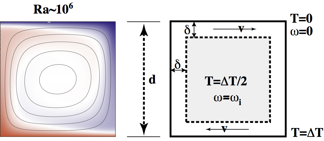
Let’s consider fully developed convection with high Rayleigh number. From observations of real fluids in laboratory situations, it is well known how this looks. High Rayleigh number convection is dominated by the advection of heat. Diffusion is too slow to carry heat far into the fluid before the buoyancy anomaly becomes unstable. This leads to thin, horizontal boundary layers where diffusive heat transfer into and out of the fluid occurs. These are separated by approximately isothermal regions in the fluid interior. The horizontal boundary layers are connected by vertical boundary layers which take the form of sheets or cylindrical plumes depending on a number of things including the Rayleigh number. For the time being we consider only the sheet like downwellings since that allows us to continue working in 2D.
Boundary layer analysis is a highly sophisticated field, and is used in a broad range of situations where differences in scales between different physical effects produce narrow accommodation zones where the weaker term dominates (e.g viscosity in an otherwise invicid flow around an obstacle).
Here we first make a wild stab at an approximate theory describing the heat flow from a layer with a given Rayleigh number. The convective flow is shown in the Figure together with a rough sketch of what actually happens.
Assuming the simplified flow pattern of the sketch, steady state, and replacing all derivatives by crude differences we obtain (using a vorticity form)
\begin{equation} \nonumber \kappa \nabla^2 T = (\mathbf{v} \cdot \nabla) T \;\;\; \longrightarrow \;\;\; \frac{v \Delta T}{d} \sim \frac{\Delta T \kappa}{\delta^2} \end{equation} and \begin{equation} \nonumber \nabla^2 \omega = \frac{g \rho \alpha}{\eta} \frac{\partial T}{\partial x} \;\;\; \longrightarrow \;\;\; \frac{\omega}{\delta ^2} \sim \frac{g \rho \alpha \Delta T}{\eta \delta} \end{equation} where \(\omega\sim v / d \) from the local rotation interpretation of vorticity and the approximate rigid-body rotation of the core of the convection cell, and \(v/d \sim \kappa / \delta^2\).
This gives
\begin{align}
\frac{\delta}{d} & \sim {\rm Ra}^{-1/3} \
v & \sim \frac{\kappa}{d} {\rm Ra}^{2/3}
\end{align}
This theory balances diffusion of vorticity and temperature across and out of the boundary layer with advection of each quantity along the boundary layer to maintain a steady state.The Nusselt number is the ratio of advected heat transport to that purely conducted in the absence of fluid motion, or, using the above approximations,
\begin{equation} \nonumber
\begin{split}
{\rm Nu} & \sim \frac{\rho C_p v \Delta T \delta}{(k \Delta T/d)d} \
& \sim {\rm Ra}^{1/3}
\end{split}
\end{equation}
This latter result being observed in experiments to be in reasonably good agreement with observation. If we define a boundary Rayleigh number \begin{equation} \nonumber {\rm Ra_b} = \frac{g \rho \alpha \Delta T \delta^3}{\kappa \eta} \end{equation} then the expression for \(\delta\) gives \begin{equation} \nonumber {\rm Ra_b} \sim 1 \end{equation}
so the boundary layer does not become more or less stable with increasing Rayleigh number (this is not universal – for internal heating the boundary layer becomes less stable at higher Rayleigh number).
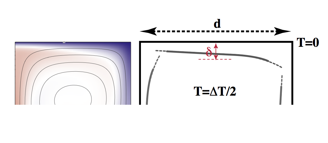
Another wrinkle can be added to the boundary layer theory by trying to account for the variation in the boundary layer thickness as it moves along the horizontal boundary. This refinement in the theory can account for the form of this thickness, the potential energy change in rising or sinking plumes, and the aspect ratio of the convection (width to height of convection roll) by maximizing Nusselt number as a function of aspect ratio.
Consider the boundary layer to be very thin above the upwelling plume (left side). As it moves to the right, it cools and the depth to any particular isotherm increases (this is clearly seen in the simulation). This can be treated exactly like a one dimensional problem if we work in the Lagrangian frame of reference attached to the boundary layer. That is, take the 1D half-space cooling model and replace the time with \(x_1/v\) (cf. the advection equation in which time and velocity / lengths are mixed).
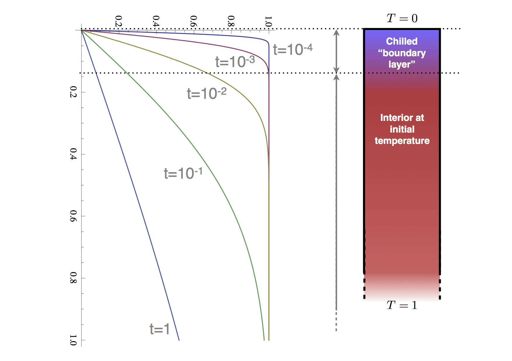
The standard solution is as follows. Assume a half-space at an intial temperature everywhere of \(T_0 \) to which a boundary condition, \(T=T_s\) is applied at \(t=0,x_2=0\).
We solve for \(T(x_2,t)\) by first making a substitution,
\begin{equation} \nonumber \theta = \frac{T-T_0}{T_s-T_0} \end{equation}
which is a dimensionless temperature, into the standard diffusion equation to obtain \begin{equation} \frac{\partial \theta(x_2,t)}{\partial t} = \kappa \frac{\partial ^2 \theta(x_2,t)}{\partial {x_2}^2} \label{eq:difftheta} \end{equation}
The boundary conditions on \(\theta\) are simple:
\begin{align}
& \theta(x_2,0) = 0 \
& \theta(0,t) = 1 \
& \theta(\infty,0) = 0
\end{align}
In place of \(t,x_2\), we use the similarity transformation,
\begin{equation} \nonumber \eta = \frac{x_2}{2\sqrt{\kappa t}} \end{equation} which is found (more or less) intuitively.
Now we need to substitute
\begin{align}
\frac{\partial \theta}{\partial t} & = -\frac{d \theta}{d\eta}(\eta/2t)
\frac{\partial^2 \theta}{\partial {x_2}^2} & = \frac{1}{4\kappa t}\frac{d^2 \theta}{d \eta^2}
\end{align}
to transform \( (\ref{eq:difftheta}) \) into
\begin{equation}
-\eta \frac{d \theta}{d\eta} = \frac{1}{2} \frac{d^2 \theta}{d \eta^2}
\label{eq:diffode}
\end{equation}
Boundary conditions transform to give
\begin{align}
& \theta(\eta=\infty) = 0
& \theta(\eta=0) = 1
\end{align}
Write \(\phi = d\theta / d\eta\) (for convenience only) to rewrite \( (\ref{eq:diffode}) \) as
\begin{align}
-\eta \phi &= \frac{1}{2} \frac{d \phi}{d \eta}
\text{or}
-\eta d\eta &= \frac{1}{2} \frac{d\phi}{\phi}
\end{align}
This is a standard integral with solution
\begin{align}
& -\eta^2 = \log_e \phi -\log_e c_1
\text{such that}
& \phi = c_1 \exp(-\eta^2) = \frac{d\theta}{d\eta}
\end{align}
This latter form is then integrated to give the solution: \begin{equation} \nonumber \theta = c_1 \int_0^\eta \exp(-{\eta’}^2) d\eta’ +1 \end{equation}
Boundary conditions give \begin{equation} \nonumber \theta = 1- \frac{2}{\sqrt{\pi}} \int_0^\eta\exp(-{\eta’}^2) d\eta’ \end{equation}
Which is the definition of the complementary error function ( \(\erfc(\eta)\)). Undoing the remaining substitutions gives \begin{equation} \nonumber \frac{T-T_0}{T_s-T_0} = \erfc \left( \frac{x_2}{2\sqrt{\kappa t}} \right) \end{equation}
In our original context of the cooling boundary layer, then, \(T _ s\) is the surface temperature, \(T_0$\) is the interior temperature of the convection cell ( \(\Delta T /2 \) ) and \(t \leftarrow x_1/v \). The thickness of the boundary layer is found by assuming it is defined by a characteristic isotherm (doesn’t much matter which). The progression of this isotherm is
\begin{equation} \nonumber
\delta \propto \sqrt{\kappa t}
\end{equation}
or, in the Eulerian frame,
\begin{equation} \nonumber
\delta \propto \sqrt{\kappa x_1 / v}
\end{equation}
Internal Heating
The definition of the Rayleigh number when the layer is significantly internally heated is
\begin{equation} \nonumber {\rm Ra} = \frac{g \rho^2 \alpha H d^5}{\eta \kappa k} \end{equation}
where \(H \) is the rate of internal heat generation per unit mass.
The definition of the Nusselt number is the heat flow through the upper surface divided by the average basal temperature. This allows a Nusselt number to be calculated for internally heated convection where the basal temperature is not known a priori. Internally heated convection is a problem to simulate in the lab, directly, but the same effect is achieved by reducing the temperature of the upper surface as a function of time.
When Viscosity is not Constant
When viscosity is not constant (and for rocks, the strong dependence of viscosity on temperature makes this generally the case), the equations are quite a lot more complicated. It is no longer possible to form the biharmonic equation since \(\eta(x,z)\) cannot be taken outside the differential operators. Nor can stream-function / vorticity formulations be used directly for the same reasons. Spectral methods — the decomposition of the problem into a sum of independent problems in the wavenumber domain — is no longer simple since the individual problems are coupled, not independent.
The Rayleigh number is no longer uniquely defined for the system since the viscosity to which it refers must take some suitable average over the layer — the nature of this average depends on the circumstances. The form of convection changes since boundary layers at the top and bottom of the system (cold v hot) are no longer symmetric with each other.
The convecting system gains another control parameter which is a measure of the viscosity contrast as a function of temperature.
Applications to the Earth
The application of realistic convection models to the Earth and other planets — particularly Venus..
The simplest computational and boundary layer solutions to the Stokes’ convection equations made the simplifying assumption that the viscosity was constant. Despite the experimental evidence which suggests viscosity variations should dominate in the Earth, agreement with some important observations was remarkably good.
Such simulations were not able to produce plate-like motions at the surface (instead producing smoothly distributed deformation) but the average velocity, the heat flow and the observed pattern of subsidence of the ocean floor were well matched.
Mantle Rheology
Experimental determination of the rheology of mantle materials gives
\begin{equation} \nonumber \dot{\epsilon} \propto \sigma^n d^{-m} \exp\left( -\frac{E+PV}{RT} \right) \end{equation}
where \(\sigma\) is a stress, \(d \) is grain size, \(E \)is an activation energy, \(V \) is an activation volume, and \(T\) is absolute temperature. ( \(R \) is the universal gas constant). This translates to a viscosity
\begin{equation} \nonumber \eta \propto \sigma^{1-n} d^m exp\left( \frac{E+PV}{RT} \right) \end{equation}
In the mantle two forms of creep are dominant: dislocation creep with \(n ~ 3.0\), \(m~0\), \(E ~ 430-540 KJ/mol\), \(V ~ 10 - 20 cm^3/mol \); and diffusion creep with \(n ~ 1.0 \), \(m~2.5\), \(E ~ 240-300 KJ/mol\), \(V ~ 5-6 cm^3/mol\). This is for olivine — other minerals will produce different results, of course.
Convection with Temperature Dependent Viscosity
More sophisticated models included the effect of temperature dependent viscosity as a step towards more realistic simulations. In fact, the opposite was observed: convection with temperature dependent viscosity is a much worse description of the oceanic lithosphere than constant viscosity convection. It may, however, describe Venus rather well.
Theoretical studies of the asymptotic limit of convection in which the viscosity variation becomes very large (comparable to values determined for mantle rocks in laboratory experiments) find that the upper surface becomes entirely stagnant with little or no observable motion. Vigorous convection continues underneath the stagnant layer with very little surface manifestation.
This theoretical work demonstrates that the numerical simulations are producing correct results, and suggests that we should look for physics beyond pure viscous flow in explaining plate motions.
Non-linear Viscosity and Brittle Effects
Realistic rheological laws show the viscosity may depend upon stress. This makes the problem non-linear since the stress clearly depends upon viscosity. In order to obtain a solution it is necessary to iterate velocity and viscosity until they no longer change.
The obvious association of plate boundaries with earthquake activity suggests that relevant effects are to be found in the brittle nature of the cold plates. Brittle materials have a finite strength and if they are stressed beyond that point they break. This is a familiar enough property of everyday materials, but rocks in the lithosphere are non-uniform, subject to great confining pressures and high temperatures, and they deform over extremely long periods of time. This makes it difficult to know how to apply laboratory results for rock breakage experiments to simulations of the plates.
An ideal, very general rheological model for the brittle lithosphere would incorporate the effects due to small-scale cracks, faults, ductile shear localization due to dynamic recrystalization, anisotropy (… kitchen sink). Needless to say, most attempts to date to account for the brittle nature of the plates have greatly simplified the picture. Some models have imposed weak zones which represent plate boundaries, others have included sharp discontinuities which represent the plate-bounding faults, still others have used continuum methods in which the yield properties of the lithosphere are known but not the geometry of any breaks. Of these approaches, the continuum approach is best able to demonstrate the spectrum of behaviours as convection in the mantle interacts with brittle lithospheric plates. For studying the evolution of individual plate boundaries methods which explicitly include discontinuities work best.
The simplest possible continuum formulation includes a yield stress expressed as an non-linear effective viscosity.
\begin{equation} \nonumber \eta _ {\rm eff} = \frac{\tau _ {\rm yield}}{\dot{\varepsilon}} \end{equation}
This formulation can be incorporated very easily into the mantle dynamics modeling approach that we have outlined above as it involves making modifications only to the viscosity law. There may be some numerical difficulties, however, as the strongly non-linear rheology can lead to dramatic variations in the viscosity across relatively narrow zones.
Thermochemical Convection
The Rayleigh number is defined in terms of thermal buoyancy but other sources of buoyancy are possible in fluids. For example, in the oceans, dissolved salt makes water heavy. When hot salty water (e.g. the outflows of shallow seas such as the Mediterranean) mixes with cold less salty water, there is a complicated interaction.
This is double diffusive convection and produces remarkable layerings etc since the diffusion coefficients of salt and heat are different by a factor of 100. In the mantle, bulk chemical differences due to subduction of crustal material can be treated in a similar manner. From the point of view of the diffusion equations, the diffusivity of bulk chemistry in the mantle is tiny (pure advection).
Fluid flows with chemical v. thermal bouyancy are termed thermochemical convection problems.