Computational Geodynamics: Miscellaneous

Sections

• 1 - Introduction
• 2 - Mathematics
• 3 - Convection
• 4 - Other Solutions

\[ \require{color} \newcommand{\dGamma}{\mathbf{d}\boldsymbol{\Gamma}} \newcommand{\erfc}{\mbox{\rm erfc}} \newcommand{\Red}[1]{\textcolor[rgb]{0.7,0.0,0.0}{#1}} \newcommand{\Green}[1]{\textcolor[rgb]{0.0,0.7,0.0}{ #1}} \newcommand{\Blue}[1]{\textcolor[rgb]{0.0,0.0,0.7}{ #1}} \newcommand{\Emerald}[1]{\textcolor[rgb]{0.0,0.7,0.3}{ #1}} \]

---

Rayleigh-Taylor Instability & Diapirism

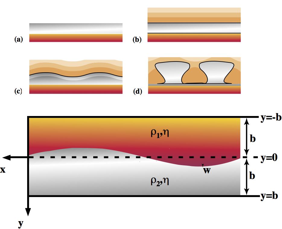
Diapirism is the buoyant upwelling of rock which is lighter than its surroundings. This can include mantle plumes and other purely thermal phenomena but it often applied to compositionally distinct rock masses such as melts infiltrating the crust (in the Archean) or salt rising through denser sediments.

Salt layers may result from the evaporation of seawater. If subsequent sedimentation covers the salt, a gravitionally unstable configuration results with heavier material (sediments) on top of light material (salt). The rheology of salt is distinctly non-linear and also sensitive to temperature. Once buried, the increased temperature of the salt layer causes its viscosity to decrease to the point where instabilities can grow. Note, since there is always a strong density contrast between the two rock types, the critical Rayleigh number argument does not apply – this situation is always unstable, but instabilities can only grow at a reasonable rate once the salt has become weak.

The geometry is outlined above in the Figure above . We suppose initially that the surface is slightly perturbed with a form of

\begin{equation} \nonumber w_m = w_{m0} \cos kx \end{equation}

where \( k \) is the wavenumber, \( k=2\pi / \lambda \), \( \lambda \) being the wavelength of the disturbance. We assume that the magnitude of the disturbance is always much smaller than the wavelength.

The problem is easiest to solve if we deal with the biharmonic equation for the stream function. Experience leads us to try to separate variables and look for solutions of the form

\begin{equation} \nonumber \psi = \left( A \sin kx + B \cos kx \right ) Y(y) \end{equation}

where the function $Y$ is to be determined. The form we have chosen for \(w_m\) in fact means $A=1,B=0$ which we can assume from now on to simplify the algebra.

Substituting the trial solution for $\psi$ into the biharmonic equation gives

\begin{equation} \nonumber \frac{d^4 Y}{d y^4} -2k^2 \frac{d^2 Y}{dy^2} +k^4 Y = 0 \end{equation}

which has solutions of the form

\begin{equation} \nonumber Y = A \exp(m y) \end{equation}

where $A$ is an arbitrary constant. Subtituting gives us an equation for $m$ \begin{equation} \nonumber m^4 - 2 k^2 m^2 + k^4 = (m^2 - k^2)^2 = 0 \label{eq:diapaux} \end{equation}
or

\begin{equation} \nonumber m = \pm k \end{equation}

Because we have degenerate eigenvalues (i.e. of the four possible solutions to the auxilliary equation (\ref{eq:diapaux}), two pairs are equal) we need to extend the form of the solution to

\begin{equation} \nonumber Y = (By+A) \exp(m y) \end{equation}

to give the general form of the solution in this situation to be

\begin{equation} \psi = \sin kx \left ( A e ^ {- ky} + B y e ^ {- ky} + C e ^ {ky} + D y e ^ {ky} \right ) \end{equation}

or, equivalently,

\begin{equation} \psi = \sin kx \left ( A _ 1 \cosh ky + B _ 1 \sinh ky + C _ 1 y \cosh ky + D _ 1 y \sinh ky \right ) \end{equation}

\label{eq:biharmsoln1}
\textrm{or, equivalently} \psi &= \sin kx \left ( A _ 1 \cosh ky + B _ 1 \sinh ky + C _ 1 y \cosh ky + D _ 1 y \sinh ky \right ) \label{eq:biharmsoln2}

This equation applies in each of the layers separately. We therefore need to find two sets of constants ${A_1,B_1,C_1,D_1}$ and ${A_2,B_2,C_3,D_4}$ by the application of suitable boundary conditions. These are known in terms of the velocities in each layer, $\mathbf{v}_1 = \mathbf{i} u_1 +\mathbf{j} v_1$ and $\mathbf{v}_2 = \mathbf{i} u_2 +\mathbf{j} v_2$:

\begin{align} u_1 = v_1 &= 0 \;\;\; \text{ on } \;\;\; y = -b \
u_2 = v_2 &= 0 \;\;\; \text{ on } \;\;\; y = b \end{align}

together with a continuity condition across the interface (which we assume is imperceptibly deformed}

\[ \begin{equation} \nonumber u_1 = u_2 \;\;\; \text{ and } \;\;\; v_1 = v_2 \;\;\; \text{ on } \;\;\; y = 0 \end{equation} \]

The shear stress (\( \sigma_{xy}\) ) should also be continuous across the interface, which, if we assume equal viscosities, gives

\begin{equation} \nonumber \frac{\partial u_1}{\partial y} + \frac{\partial v_1}{\partial x} = \frac{\partial u_2}{\partial y} + \frac{\partial v_2}{\partial x} \;\;\; \text{on} \;\;\; y = 0 \end{equation}

and, to simplify matters, if the velocity is continuous across $y=0$ then any velocity derivatives in the $x$ direction evaluated at $y=0$ will also be continuous (i.e. $\partial v_2 / \partial x = \partial v_1 / \partial x$). The expressions for velocity in terms of the solution (\ref{eq:biharmsoln2}) are

\begin{align} u = -\frac{\partial \psi}{\partial y} & = -\sin kx \left( (A_1 k + D_1 + C_1 k y) \sinh ky + (B_1 k + C_1 + D_1 ky) \cosh ky \right) \
v = \frac{\partial \psi}{\partial x} & = k \cos kx \left( (A_1 +C_1 y)\cosh ky + (B_1 +D_1 y) \sinh ky \right) \end{align}

From here to the solution requires much tedious rearrangement, and the usual argument based on the arbitrary choice of wavenumber $k$ but we finally arrive at

\begin{multline} \psi_1 = A_1 \sin kx \cosh ky + \
A_1 \sin kx \left[ \frac{y}{k b^2} \tanh kb \sinh ky + \left( \frac{y}{b} \cosh ky \frac{1}{kb} \sinh ky \right) \cdot \left( \frac{1}{kb} + \frac{1}{\sinh bk \cosh bk} \right) \right] \times \
\left[ \frac{1}{\sinh bk \cosh bk} - \frac{1}{(b^2k^2} \tanh bk \right] ^{-1} \label{eq:raytays1} \end{multline}

The stream function for the lower layer is found by replacing $y$ with $-y$ in this equation. This is already a relatively nasty expression, but we haven’t finished since the constant $A_1$ remains. This occurs because we have so far considered the form of flows which satisfy all the boundary conditions but have not yet considered what drives the flow in each layer.

To eliminate $A_1$, we have to consider the physical scales inherent in the problem itself. We are interested (primarily) in the behaviour of the interface which moves with a velocity $\partial w / \partial t$. As we are working with small deflections of the interface,

\begin{equation} \nonumber \frac{\partial w}{\partial t} = \left. v \right| _ {y=0} \end{equation}

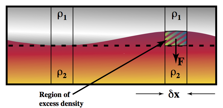
Consider what happens when the fluid above the interface is lighter than the fluid below – this situation is stable so we expect the layering to be preserved, and if the interface is disturbed the disturbance to decay. This implies that there must be a restoring force acting on an element of fluid which is somehow displaced across the boundary at $y=0$ (Figure above).

This restoring force is due to the density difference between the displaced material and the layer in which it finds itself. The expression for the force is exactly that from Archimedes principle which explains how a boat can float (only in the opposite direction)

\begin{equation} \nonumber \left. F_2 \right|_{y=0} = \delta x g w (\rho _ 2 - \rho _ 1) \end{equation}

which can be expressed as a normal stress difference (assumed to apply, once again, at the boundary). The viscous component of the normal stress turns out to be zero – proven by evaluating $\partial v / \partial y$ at $y=0$ using the expression for \( \phi \) in equation (\ref{eq:raytays1}). Thus the restoring stress is purely pressure

\[ \begin{equation} \nonumber \left. P_2 \right|_{y=0} = g w (\rho_2 - \rho_1) \end{equation} \]

The pressure in terms of the solution (so far) for $\psi$ is found from the equation of motion in the horizontal direction (substituting the stream function formulation) and is then equated to the restoring pressure above. \[ \begin{equation} \nonumber (\rho_1-\rho_2) g w = -\frac{4 \eta k A_1}{b} \cos kx \left(\frac{1}{kb} + \frac{1}{\sinh bk \cosh bk} \right) \cdot \left( \frac{1}{\sinh bk \cosh bk} - \frac{1}{(b^2k^2} \tanh bk \right)^{-1} \end{equation} \] which allows us to substitute for $A_1$ in our expression for $\partial w / \partial t$ above. Since $A_1$ is independent of $t$, we can see that the solution for $w$ will be of a growing or decaying exponential form with growth/decay constant coming from the argument above.

\[ \begin{equation} \nonumber w(t) = w_0 \exp((t-t_0)/\tau) \end{equation} \] where \[ \begin{equation} \nonumber \tau = \frac{4 \eta}{(\rho_1-\rho_2) g b} \left( \frac{1}{kb} + \frac{1}{\sinh bk \cosh bk} \right) \cdot \left( \frac{1}{k^2b^2} \tanh kb - \frac{1}{\sinh kb \cosh kb} \right)^{-1} \end{equation} \]

So, finally, an answer – the rate at which instabilities on the interface between two layers will grow (or shrink) which depends on viscosity, layer depth and density differences, together with the geometrical consideration of the layer thicknesses.

A stable layering results from light fluid resting on heavy fluid; a heavy fluid resting on a light fluid is always unstable (no critical Rayleigh number applies) although the growth rate can be so small that no deformation occurs in practice. The growth rate is also dependent on wavenumber. There is a minimum in the growth time as a function of dimensional wavenumber which occurs at $k b = 2.4$, so instabilities close to this wavenumber are expected to grow first and dominate.

Remember that this derivation is simplified for fluids of equal viscosity, and layers of identical depth. Remember also that the solution is for {\rm infinitessimal} deformations of the interface. If the deformation grows then the approximations of small deformation no longer hold. This gives a clue as to how difficulties dealing with the advection term of the transport equations arise. At some point it becomes impossible to obtain meaningful results without computer simulation. However, plenty of further work has already been done on this area for non-linear fluids, temperature dependent viscosity \&c and the solutions are predictably long and tedious to read, much less solve. When the viscosity is not constant, the use of a stream function notation is not particularly helpful as the biharmonic form no longer appears. \Emerald{(e.g. read work by Ribe, Houseman et al.)}

The methodology used here is instructive, as it can be used in a number of different applications to related areas. The equations are similar, the boundary conditions different.

Post-Glacial Rebound

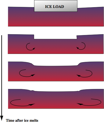
In the postglacial rebound problem, consider a viscous half space with an imposed topography at $t=0$. The ice load is removed at $t=0$ and the interface relaxes back to its original flat state.

This can be studied one wavenumber at a time — computing a decay rate for each component of the topography. The intial loading is computed from the fourier transform of the ice bottom topography. The system is similar to that of the diapirs except that the loading is now applied to one surface rather than the interface between two fluids.

Phase Changes in the mantle

A different interface problem is that of mantle phase changes. Here a bouyancy anomaly results if the phase change boundary is distorted. This can result from advection normal to the boundary bringing cooler or warmer material across the boundary.

The buoyancy balance argument used above can be recycled here to determine a scaling for the ability of plumes/downwellings to cross the phase boundary.

Sensitivity Kernels for Surface Observables

The solution method used for the Rayleigh Taylor problem can also be used in determining spectral Green’s functions for mantle flow in response to thermal perturbations. This is a particularly abstract application of the identical theory.

Folding of Layered (Viscous) Medium

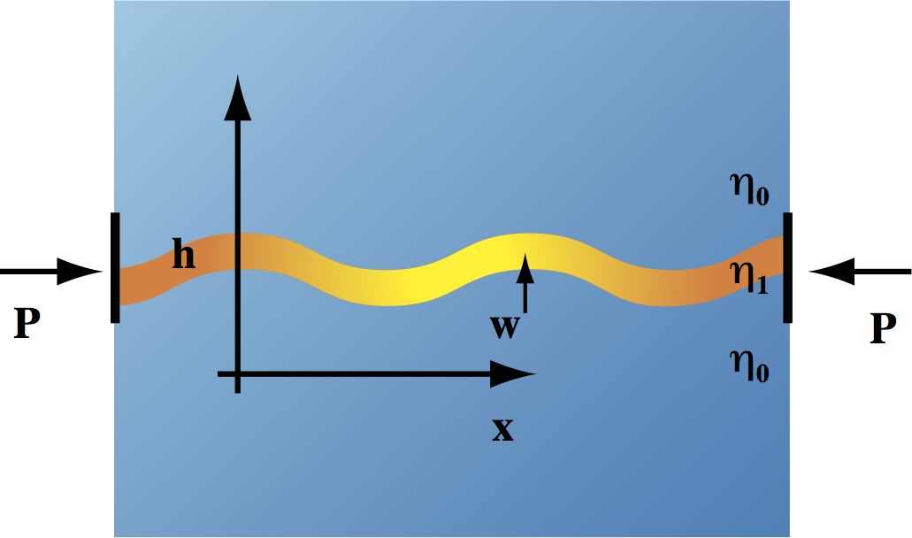
If a thin viscous layer is compressed from one end then it may develop buckling instabilities in which velocities grow perpendicular to the plane of the layer. If the layer is embedded between two semi-infinite layers of viscous fluid with viscosity much smaller than the viscosity of the layer, then Biot theory tells us the wavelength of the initial buckling instability, and the rate at which it grows.

The fold geometry evolves as \[ \begin{equation} \nonumber w=w_m \cos(kx) e^{\frac{t}{\tau_a}} \end{equation} \] where \[ \begin{equation} \nonumber \tau_a = \frac{1}{\bar{P}}\left[ \frac{4 \eta_0}{k} + \frac{\eta_1 h^3}{3k^2} \right] \end{equation} \] and the fastest growing wavenumber is \[ \begin{equation} \nonumber k = \frac{6}{h}\left( \frac{\eta_1}{\eta_0} \right)^{\frac{1}{3}} \end{equation} \]

For large deformations we eventually must resort to numerical simulation.

Gravity Currents

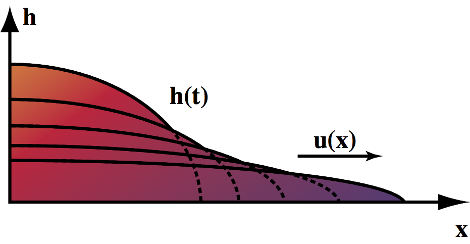
Gravity currents can occur when a viscous fluid flows under its own weight as shown in the Figure above.

We assume that the fluid has constant viscosity, $\eta$ and that the length of the current is considerably greater than its height. The fluid is embedded in a low viscosity medium of density $\rho-\Delta \rho$ where $\rho$ is the density of the fluid itself.

The force balance is between buoyancy and viscosity. The assumptions of geometry allow us to simplify the Stokes equation by assuming horizontal pressure gradients due to the surface slope drive the flow.

\[ \begin{equation} \nonumber \nabla p = \eta\nabla^2 u \approx g \Delta \rho \frac{\partial h}{\partial x}
\end{equation} \]

We assume near-zero shear stress at the top of the current to give \[ \begin{equation} \nonumber \frac{\partial u}{\partial z} (x,h,t) = 0 \end{equation} \] and zero velocity at the base of the current. Hence \[ \begin{equation} \nonumber u(x,z,t) = -\frac{1}{2} \frac{g \Delta \rho}{\eta} \frac{\partial h}{\partial x} z(2h-z) \end{equation} \]

Continuity integrated over depth implies \[ \begin{equation} \nonumber \frac{\partial h}{\partial t} + \frac{\partial }{\partial x} \int_0^h u dz = 0 \end{equation} \] Combining these equations gives \[ \begin{equation} \nonumber \frac{\partial h}{\partial t} -\frac{1}{3} \frac{g \Delta \rho}{\eta} \frac{\partial }{\partial x} \left( h^3 \frac{\partial h}{\partial x} \right) = 0 \end{equation} \] Finally, a global constraint fixes the total amount of fluid at any given time \[ \begin{equation} \nonumber \int_0^{x_N(t)} h(x,t)dx = qt^\alpha \end{equation} \] The latter term being a fluid source at the origin, and $x_ {N(t)}$ the location of the front of the current. A similarity variable can be used to transform this problem: \[ \begin{equation} \nonumber \nu = \left( \frac{1}{3} g\Delta \rho q^3 / \eta \right)^{-\frac{1}{5}} x t^{-(3\alpha +1) / 5} \end{equation} \] giving a solution of the form \[ \begin{equation} \nonumber h(x,t) = \nu_N^{2/3} (3q^2 \eta / (g\Delta\rho))^{1/5} t^{(2\alpha -1) / 5} \phi(\nu/\nu_N) \end{equation} \] where $\nu_N$ is the value of $\nu$ at $x=x_N(t)$. Substituting into the equation for $\partial h / \partial t$ we find that $\phi(\nu/\nu_N)$ satisfies \[ \begin{equation} \nonumber \phi({\nu}/{\nu_N}) = \left[ \frac{3}{5}(3\alpha+1)\right]^{\frac{1}{3}} \left(1-\frac{\nu}{\nu_N} \right)^{\frac{1}{3}} \left[ 1 - \frac{3\alpha-4}{24(3\alpha+1)}\left(1-\frac{\nu}{\nu_N} \right) + O \left(1-\frac{\nu}{\nu_N} \right)^2 \right] \end{equation} \] Which has an analytic solution if $\alpha=0$ (only constant sources or sinks) \[ \begin{equation} \nonumber \begin{split} \phi({\nu}/{\nu_N}) &= \left( \frac{3}{10}\right)^{\frac{1}{3}} \left( 1-\left(\frac{\nu}{\nu_N}\right)^2 \right)^{\frac{1}{3}}
\nu_N &= \left[ \frac{1}{5} \left( \frac{3}{10}\right)^{\frac{1}{3}} \pi^{\frac{1}{2}} \Gamma (1/3) / \Gamma (5/6) \right]^{-\frac{3}{5}} = 1.411 \end{split} \end{equation} \] For all other values of $\alpha$ numerical integration schemes must be used for \( \phi \). It is also possible to obtain solutions if axisymmetric geometry is used.

---