

Computational Geodynamics: Decay Equation
\[ \newcommand{\dGamma}{\mathbf{d}\boldsymbol{\Gamma}} \newcommand{\erfc}{\mbox{\rm erfc}} \newcommand{\curly}{\sf } \newcommand{\Red }[1]{\textcolor[rgb]{0.7,0.0,0.0}{ #1}} \newcommand{\Green }[1]{\textcolor[rgb]{0.0,0.7,0.0}{ #1}} \newcommand{\Blue }[1]{\textcolor[rgb]{0.0,0.0,0.7}{ #1}} \newcommand{\Emerald }[1]{\textcolor[rgb]{0.0,0.7,0.3}{ #1}} \]
Sections
We start with the numerical solution of a very simple differential equation. In fact we choose something simple enough that we already know the answer.
\begin{equation} \frac{d\theta}{dt} = - k \theta \label{eq:ode_decay} \end{equation}
This is the equation which governs radioactive decay, in which case \(\theta \) is the amount of the radioactive isotope remaining and \(d\theta / dt\) is the activity that we can measure. \(k\) is closely related to the half life.
The solution to this equation is \[ \theta(t) = \theta_0 e^{-kt} \] where \(\theta_0\) is the amount of the radioactive material remaining. The same equation also describes the cooling of, say, a cup of coffee. In this case we interpret \(\theta \) as the excess temperature (above room temperature).
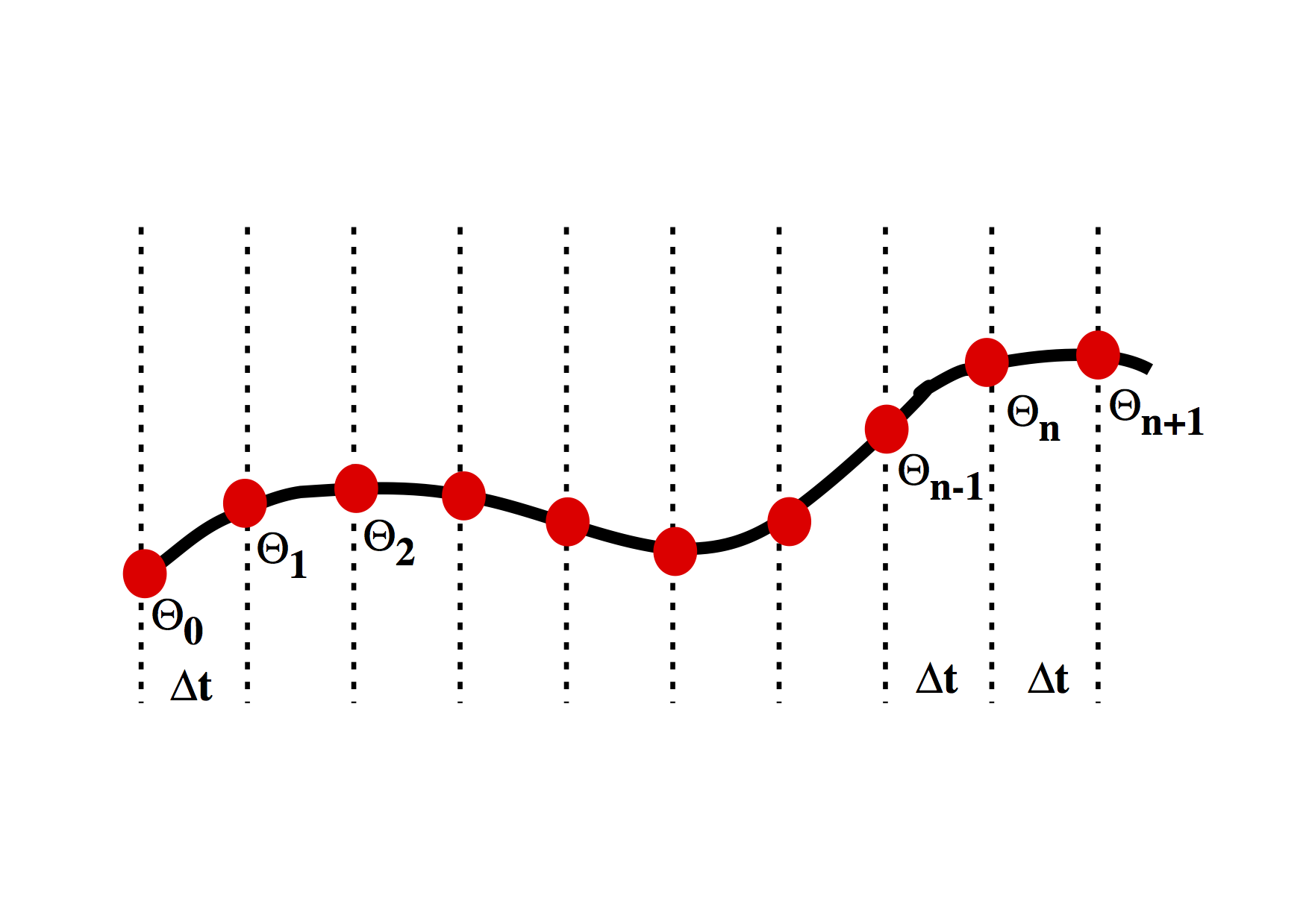
We want to march forward in time from our starting point where \(\theta = \theta_0\) to obtain the value of \( \theta \) at later times. To do this, we need to approximate the original differential equation, and, in particular, the value of the time derivative at each time. There are a number of ways to do this.
A first order numerical approximation
Assume that the variation in \(\theta(t) \) is linear, i.e.
\[
\theta(t’) = \theta _ n + \beta t’
\]
where we use a local time coordinate \(t’ = t - n\Delta t\), so that when we differentiate
\[
\frac{d \theta}{dt} = \beta
\]
To determine the approximation for the derivative therefore becomes the solution to the following equation:
\[
\begin{split}
& \theta _ {n+1} = \theta _ n + \beta \Delta t
& \Rightarrow \beta = \frac{d \theta}{dt} = \frac{\theta _ {n+1} - \theta _ n}{\Delta t}
\end{split}
\]
This is a first order difference expression for the derivative which we substitute into the original differential equation (\( \ref{eq:ode_decay}\) ) at the current timestep \[ \frac{\theta _ {n+1} - \theta _ n}{\Delta t} = - k \theta _ n \]
This rearranges to give us a time-marching algorithm:
\[ \theta _ {n+1} = \theta _ n (1-k \Delta t) \]
It is an indication of the fact that this problem is really not all that difficult that this difference equation can be written recursively to give: \[ \theta_{n+1} = \theta_0 (1-k \Delta t)^n \] In a moment we will compute some values for this expression to see how accurate it is. First we consider whether we can improve the accuracy of the approximation by doing a bit more work.
Higher order expansion
First we try fitting the local expansion for \(\theta \) through an additional point. This time we assume that the variation in \(\theta(t)\) is quadratic, i.e. \[ \theta(t’) = \theta _ {n-1} + \beta t’ + \gamma {t’}^2 \] The local time coordinate is \(t’ = t - (n-1)\Delta t \), and when we differentiate \begin{equation} \frac{d \theta}{dt} = \beta + 2 \gamma t’ \label{eq:dthdt2} \end{equation}
To solve for \(\beta \) and \(\gamma \) we fit the curve through
the sample points:
\[
\begin{split}
\theta _ n &= \theta _ {n-1} + \beta \Delta t + \gamma (\Delta t)^2
\theta _ {n+1} &= \theta _ {n-1} + 2 \beta \Delta t + 4 \gamma (\Delta t)^2
\end{split}
\]
Which we can solve to give this:
\[
\begin{split}
\beta &= \left( 4 \theta _ n - \theta_{n+1} - 3\theta _ {n-1} \right) \frac{1}{2\Delta t}
\gamma &= \left( \theta _ {n+1} + \theta _ {n-1} -2 \theta _ n \right) \frac{1}{2\Delta t^2}
\end{split}
\]
By substituting into \( (\ref{eq:dthdt2}) \), and then into the original differential equation \( (\ref{eq:ode_decay}) \) we obtain the following
\[
\left. \frac{d\theta}{dt} \right| _ {t=n\Delta t} = \beta + 2\gamma \Delta t =
\frac{1}{2\Delta t} \left( \theta _ {n+1} - \theta _ {n-1} \right) = -k \theta _ n
\]
The difference approximation to the derivative turns out to be the average of the expressions for the previous derivative and the new derivative. We have now included information about the current timestep and the previous timestep in our expression for the value of \(\theta \) at the forthcoming timestep:
\[
\theta _ {n+1} = \theta _ {n-1} -2k \theta _ n \Delta t
\]
A comparison of the two schemes
How well do these two methods perform, and what difference does the choice of \(\Delta t \) make on the accuracy ?
| t | \(^1\theta _ H\) | \(^1\theta _ h\) | \(^2\theta _ H\) | \(^2\theta _ h\) | Exact |
|---|---|---|---|---|---|
| 0.0 | 1.0000 | 1.0000 | 1.0000 | 1.0000 | 1.0000 |
| 0.1 | - | 0.9000 | - | 0.9000 | 0.9048 |
| 0.2 | 0.8000 | 0.8100 | 0.8000 | 0.8200 | 0.8187 |
| 0.3 | - | 0.7290 | - | 0.7360 | 0.7408 |
| 0.4 | 0.6400 | 0.6561 | 0.6800 | 0.6728 | 0.6703 |
| 0.5 | - | 0.5905 | - | 0.6014 | 0.6063 |
| 0.6 | 0.5120 | 0.5314 | 0.5280 | 0.5525 | 0.5488 |
| 0.7 | - | 0.4783 | - | 0.4909 | 0.4966 |
| 0.8 | 0.4096 | 0.4305 | 0.4688 | 0.4543 | 0.4483 |
| 0.9 | - | 0.3874 | - | 0.4001 | 0.4066 |
| 1.0 | 0.3277 | 0.3487 | 0.3405 | 0.3743 | 0.3679 |
Results of the numerical simulation of the decay equation. \(^1\theta_H \) is from the first order expansion of \(\theta(t) \), at a timestep of \( \Delta t=0.2 \), and \(^2\theta_H \) is the second order expansion at \( \Delta t=0.2 \); other calculations are at \(\Delta t = 0.1 \). \(^1\theta_h\) is the linear expansion, \(^2\theta_h\) results from the quadratic expansion of \(\theta(t)\). The actual solution is also shown.
The results are more accurate when a smaller timestep is used although it requires more computation to achieve the greater accuracy. Higher order expansion also increases the accuracy and may be more efficient in terms of the number of computations required for a given level of accuracy. Note, however, that the supposedly better quadratic expansion produces an error which oscillates as time increases. Does this error grow ? Does this make second order expansions useless ?
Second Order Runge-Kutta
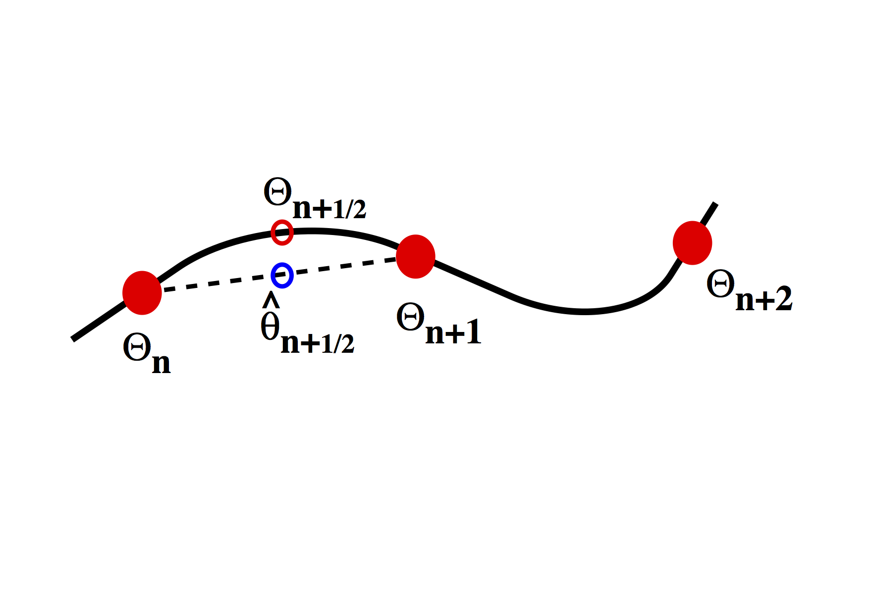
The Runge-Kutta approach to higher order integration methods is illustrated above. The idea is to estimate the gradient \(d \theta / d t\) at the half way point between two timestep values. This is done in two stages. Initially a first order estimate, \(\hat{\theta}\) is made for the value of the function \( \theta \) at \(t=t+\Delta t /2\) in the future. This value is then subsituted into the differential equation to obtain the estimate for the gradient at this time. The revised gradient is then used to update the original \(\theta(t)\) by an entire timestep.
The first order step is
\[
\begin{split}
\hat{\theta}(t+\Delta t /2) & = \theta(t) + \left. \frac{d \theta}{d t} \right| _ t \frac{\Delta t}{2}
&= \theta(t) \left[ 1-\frac{k\Delta t}{2} \right]
\end{split}
\]
Substitute to estimate the gradient at the mid-point
\[
\left. \frac{d \theta}{d t} \right| _ {t+\Delta t /2} \approx -k \theta(t) \left[ 1-\frac{k\Delta t}{2} \right]
\]
Use this value as the average gradient over the interval \( t\rightarrow t+\Delta t \) to
update \(\theta \)
\[
\begin{split}
\theta(t+\Delta t) & \approx \theta(t) + \delta t \left( -k \theta(t) \left[ 1-\frac{k\Delta t}{2} \right] \right)
& \approx \theta(t) \left( 1 - k \Delta t + k^2 \frac{\Delta t^2}{2} \right)
\end{split}
\]
It’s worth noting that the Taylor expansion of the solution should look like
\[
e^{-kt} = 1 - kt + \frac{k^2 t^2}{2!} - \frac{k^3 t^3}{3!} + \ldots
\]
The Runge Kutta method can be extended by repeating the estimates on smaller regions of the interval. The usual choice is fourth order RK. This is largely because, obviously, it’s accurate to fourth order, but also because the number of operations to go higher than fourth order is disproportionately large. See Numerical Recipes for a discussion on this and better methods for ODE’s.
Our First Code
The simplest way to answer our earlier question is to code the methods and see. The following is a script which computes the first and second order expressions and the Runge-Kutta method, and compares with the “exact” solution (which is numerical as well, of course, but computed through series expansions and the like).
# Compare various ways to integrate the
# ODE for radioactive decay / Newton's law of cooling.
# Assume decay constant of 1.0

import math

timestep=0.1;

# Initial value ...

theta1_0   = 1.0
theta2_0   = 1.0
thetaRK2_0 = 1.0

# First timestep (by hand, then automate for subsequent cases)

theta1_1   = 0.9
theta2_1   = 0.9
thetaRK_1  = 0.905

# Now we have enough information to automate all the methods

for i in range(2,1001):

    time = timestep * i
    exact = 1.0 * math.exp(-1.0 * time)

    theta1_2  = theta1_1 * (1.0 - timestep)
    theta2_2  = theta2_0 - 2.0 *  theta2_1 * timestep
    thetaRK_2 = thetaRK_1 * (1.0 - timestep + 0.5 * timestep * timestep)

  # output data every 25th step
    if not (i % 25):
        print "Timestep {:04d} {:.4f}\t {:.4e} \t {:.4e} \t {:.4e} \t {:.4e}".format(i,time,theta1_2,theta2_2,thetaRK_2,exact)

  # keep old values (not all are needed, of course)

    theta1_0  = theta1_1
    theta2_0  = theta2_1
    thetaRK_0 = thetaRK_1

    theta1_1  = theta1_2
    theta2_1  = theta2_2
    thetaRK_1 = thetaRK_2

""" Output:
Timestep 0025 2.5000     +7.1790e-02     +5.2117e-02     +8.2455e-02     +8.2085e-02
Timestep 0050 5.0000     +5.1538e-03     +3.7201e-01     +6.7987e-03     +6.7379e-03
Timestep 0075 7.5000     +3.6999e-04     -4.4304e+00     +5.6059e-04     +5.5308e-04
Timestep 0100 10.0000    +2.6561e-05     +5.3757e+01     +4.6223e-05     +4.5400e-05
Timestep 0125 12.5000    +1.9068e-06     -6.5219e+02     +3.8113e-06     +3.7267e-06
Timestep 0150 15.0000    +1.3689e-07     +7.9124e+03     +3.1426e-07     +3.0590e-07
Timestep 0175 17.5000    +9.8274e-09     -9.5993e+04     +2.5912e-08     +2.5110e-08
Timestep 0200 20.0000    +7.0551e-10     +1.1646e+06     +2.1366e-09     +2.0612e-09
Timestep 0225 22.5000    +5.0648e-11     -1.4129e+07     +1.7617e-10     +1.6919e-10
Timestep 0250 25.0000    +3.6360e-12     +1.7141e+08     +1.4526e-11     +1.3888e-11
Timestep 0275 27.5000    +2.6103e-13     -2.0796e+09     +1.1977e-12     +1.1400e-12
Timestep 0300 30.0000    +1.8739e-14     +2.5230e+10     +9.8758e-14     +9.3576e-14
Timestep 0325 32.5000    +1.3453e-15     -3.0609e+11     +8.1431e-15     +7.6812e-15
Timestep 0350 35.0000    +9.6578e-17     +3.7135e+12     +6.7143e-16     +6.3051e-16
Timestep 0375 37.5000    +6.9333e-18     -4.5052e+13     +5.5363e-17     +5.1756e-17
Timestep 0400 40.0000    +4.9774e-19     +5.4658e+14     +4.5649e-18     +4.2484e-18
Timestep 0425 42.5000    +3.5733e-20     -6.6311e+15     +3.7640e-19     +3.4873e-19
Timestep 0450 45.0000    +2.5652e-21     +8.0449e+16     +3.1036e-20     +2.8625e-20
Timestep 0475 47.5000    +1.8416e-22     -9.7602e+17     +2.5590e-21     +2.3497e-21
Timestep 0500 50.0000    +1.3221e-23     +1.1841e+19     +2.1100e-22     +1.9287e-22
Timestep 0525 52.5000    +9.4911e-25     -1.4366e+20     +1.7398e-23     +1.5832e-23
Timestep 0550 55.0000    +6.8137e-26     +1.7429e+21     +1.4346e-24     +1.2996e-24
Timestep 0575 57.5000    +4.8915e-27     -2.1144e+22     +1.1829e-25     +1.0668e-25
Timestep 0600 60.0000    +3.5116e-28     +2.5653e+23     +9.7532e-27     +8.7565e-27
Timestep 0625 62.5000    +2.5210e-29     -3.1122e+24     +8.0420e-28     +7.1878e-28
Timestep 0650 65.0000    +1.8098e-30     +3.7757e+25     +6.6310e-29     +5.9001e-29
Timestep 0675 67.5000    +1.2993e-31     -4.5807e+26     +5.4675e-30     +4.8431e-30
Timestep 0700 70.0000    +9.3273e-33     +5.5574e+27     +4.5082e-31     +3.9754e-31
Timestep 0725 72.5000    +6.6961e-34     -6.7423e+28     +3.7172e-32     +3.2632e-32
Timestep 0750 75.0000    +4.8071e-35     +8.1797e+29     +3.0650e-33     +2.6786e-33
Timestep 0775 77.5000    +3.4510e-36     -9.9237e+30     +2.5273e-34     +2.1988e-34
Timestep 0800 80.0000    +2.4775e-37     +1.2040e+32     +2.0838e-35     +1.8049e-35
Timestep 0825 82.5000    +1.7786e-38     -1.4606e+33     +1.7182e-36     +1.4815e-36
Timestep 0850 85.0000    +1.2768e-39     +1.7721e+34     +1.4167e-37     +1.2161e-37
Timestep 0875 87.5000    +9.1663e-41     -2.1499e+35     +1.1682e-38     +9.9824e-39
Timestep 0900 90.0000    +6.5805e-42     +2.6082e+36     +9.6321e-40     +8.1940e-40
Timestep 0925 92.5000    +4.7241e-43     -3.1643e+37     +7.9421e-41     +6.7261e-41
Timestep 0950 95.0000    +3.3914e-44     +3.8390e+38     +6.5486e-42     +5.5211e-42
Timestep 0975 97.5000    +2.4347e-45     -4.6575e+39     +5.3996e-43     +4.5320e-43
Timestep 1000 100.0000   +1.7479e-46     +5.6505e+40     +4.4522e-44     +3.7201e-44
"""
Clearly, the quadratic expansion does not do a good job in this particular case, since the error is a growing instability which makes the solution useless almost immediately. However, the second order Runge-Kutta method is very accurate. This gives a clear warning that numerical solution of equations is partly an art (though the stability or otherwise of a given method can actually be proven formally in many cases).
Explicit versus Implicit Methods}
The use of implicit solution methods is crucial when we come to the mantle flow problem (and to elasticity). It is a deceptively simple concept which we use to eliminate oscillatory errors and other problems associated with stiff systems, and in other cases where we want to take large timesteps. Again, Numerical Recipes provides a good example of the way in which implicit methods avoid the shuffling timesteps which result when an otherwise unimportant component of the system blows up. To obtain an implicit solution, we express our updated timestep in terms of values of derivatives etc which are evaluated at that timestep. This may result in dependencies which mean large systems of simultaneous equations need to be solved.
But our simple example can also be solved implicitly as follows
\[
\theta(t+\Delta t) = \left. \frac{d \theta}{d t} \right| _ {t+\Delta t} + \theta(t)
\]
Easy to write down, but \(\left. d \theta/ dt \right| _ {t+\Delta t}\) is not known until \(\theta(t+\Delta t) \) is known. In this case, however, we simply substitute \(\left. d \theta/ dt \right| _ {t+\Delta t}= -k \theta(t+\Delta t) \) from the differential equation and write
\[
\begin{split}
\theta(t+\Delta t) & = -k \theta(t+\Delta t) \Delta t + \theta(t)
& = \frac{\theta(t) }{ 1 + k\Delta t}
\end{split}
\]
A higher order implicit method can be found by considering how the second order Runge-Kutta method constructs its estimates. In place of the first order approximation above, we try
\[
\theta(t+\Delta t) = \left. \frac{d \theta}{d t} \right| _ {t+\Delta t/2} + \theta(t)
\]
where we assume
\[
\left. \frac{d \theta}{d t} \right| _ {t+\Delta t/2} =
\frac{1}{2} \left. \frac{d \theta}{d t} \right| _ {t+\Delta t} +
\frac{1}{2} \left. \frac{d \theta}{d t} \right| _ {t}
\]
Substituting from our original differential equation now gives
\[
\begin{split}
\theta(t+\Delta t) &= -k\frac{\theta(t+\Delta t) + \theta(t)}{2} \Delta t + \theta(t)
&= \theta(t) \frac{1-k\Delta t / 2}{1+k\Delta t / 2}
\end{split}
\]
| \(t\) | \(^1\theta_i\) | \(^2\theta_i\) | Exact |
|---|---|---|---|
| 0.0 | 1.0000 | 1.0000 | 1.0000 |
| 0.1 | 0.9091 | 0.9048 | 0.9048 |
| 0.2 | 0.8264 | 0.8186 | 0.8187 |
| 0.3 | 0.7513 | 0.7406 | 0.7408 |
| 0.4 | 0.6830 | 0.6701 | 0.6703 |
| 0.5 | 0.6209 | 0.6063 | 0.6063 |
Results of the two implicit schemes derived above for the numerical integration of the decay equation
The first order scheme is of approximately the same accuracy as the explicit scheme, not surprisingly, but the mid-point implicit method has very impressive results considering that there is very little extra work involved in deriving the formulation. Can this strategy stabilize the quadratic expansion which proved to be so unstable in explicit form ? Evaluating the derivatives at time \(t=(n+1)\Delta t\) gives
\[ \left. \frac{d \theta}{d t} \right| _ {(n+1)\Delta t} = 3 \theta _ {n+1} - 4\theta _ n + \theta _ {n-1} \]
which we substitute into the differential equation at \(t=(n+1)\Delta t\) to give (eventually)
\[ \theta _ {n+1} = \frac{4\theta _ n - \theta _ {n-1}}{3+2k\Delta t} \]
This method is stable although not as accurate as the second order Runge-Kutta Scheme. It is trivial to modify the Python script to demonstrate this.
References
…